Ted Papalexopoulos · December 9, 2021
This post serves as an explainer of the paper of the same name by Vlastelica et al., published as a conference paper at ICLR 2020 [1]. It was written as a final project for the Fall 2021 seminar 6.S898: Deep Learning at the Massachusetts Institute of Technology. Needless to say that the exposition and intuition herein is heavily adapted by the paper itself.
I probably won't be accused of being controversial when I say that deep learning has revolutionized predictive analytics. Deep nets of all kinds of flavours have emerged as state of the art models in domains ranging from object detection to machine translation. Much has been made of NNs' ability to scalably and reliably extract rich feature representations from low-level data, e.g. raw images or text, and thus achieve prediction accuracies that are often orders of magnitude higher than traditional learning approaches.
It is important to keep in mind, however, that accurate prediction is rarely the end goal for practitioners. The label of prescriptive analytics has recently gained popularity, as a way to express the fundamental (if self-evident) fact that predictions are merely a means to an end. The reason we predict future behaviour is so that we can make better decisions in the present. Companies use demand predictions to decide how much product to produce or how much inventory to stock. Self-driving cars predict a pedestrian's movements to decide whether to slow down. Transplant hospitals predict how likely a patient is to die to decide how to allocate recovered organs. After prediction, comes prescription.
This simple fact has inpired an abundance of research on machine learning methods that are "aware" of the downstream prescription task, and seek to directly obtain high-quality decisions instead of naively minimizing the intermediate prediction error. The focus of this post is one of many such approaches, based on the paper Differentiation of Blackbox Combinatorial Solvers [1].
As the title suggests, the paper proposes a principled mechanism to differentiate through a general class of combinatorial optimization solvers. The upshot is that any such solver can then be plugged into neural architecture that remains differentiable, and hence trainable using standard back propagation. Crucially, the backward pass through the solver layer requires just one additional call to the solver, and so its compuational cost is the same as the forward pass.
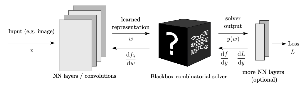
We'll deconstruct how it all works shortly, but let's first understand what such an architecture (pictured below) looks like, and why it might be useful.
Starting from the left, a raw input representation \(x\) is transformed according to some NN architecture \(-\) this can be a convolutional network, transformer, graph neural network etc. Its output \(w\) is a learned representation of (unknown) parameters in some optimization problem for which we have a custom solver, namely a function that maps \(w\) to the optimal solution \(y(w)\) over some domain \(Y\):
\[y(w) = \underset{y \in Y}{\arg\min} \; c(w, y)\]
The optimized solution \(y(w)\) (or some further modified representation of it) is the final output of the architecture. In a sense, this is a "hybrid" predictive/prescriptive architecture in that it (i) predicts some uncertain parameters \(w\), and (ii) prescribes an optimal decision under \(w\) by solving an optimization problem. For training we of course need to define a loss function \(L\), called the decision loss, which codifies how good the decision is.
As an illustrative example, which I'll keep coming back to, let's consider a ubiquitous problem solved millions of times every day by Google Maps. Given an origin and destination location, we wish to find a driving route connecting them with minimum travel time. Mathematically, this corresponds to finding the shortest path on a graph representing the road network, where nodes are intersections, edges are roads, and edge costs are travel times.

Note how there's a (not very well) hidden prediction problem that comes before prescription: for each edge, we need to know how long it will take us to traverse it, if and when we pass through it.
That's where an architecture such as Figure 1 comes in. We might start with input data \(x\) representing low-level node/edge information from live traffic data, e.g. the number of cars on each road and their average speeds. Some sub-architecture, e.g. a Graph Convolution Network, outputs edge representations \(w\) that we hope will learn to encode travel times using pooled information from local graph neighborhoods. The predicted edge costs are passed as input to Dijkstra's algorithm or some other solver, which computes the corresponding shortest path \(y(w)\) between origin and destination. And finally, for supervised training, the decision error \(L(y(w))\) of the prescribed path is computed, e.g. its Hamming Distance from the true shortest path (which we would know after observing the true traffic).
I probably don't need to convince you that using an NN to predict edge costs is a good idea; NNs can extract rich feature representations, pool information according to the local graph structure etc. The question I do want to focus on for a second is:
Why should we want to build the optimization into the NN itself?
In other words, why might we expect a hybrid architecture to perform better than a two-stage approach where we (i) train a vanilla NN to minimize prediction error on \(w\) (e.g., the \(\ell_2\) loss), using the the same pre-solver architecture, and (ii) plug the predictions into the solver to get our prescription. This framework is often called "predict-then-optimize" (don't you just love the creativity?) and is simple enough to be the thing anyone should try.
As one might expect, however, it can leave a lot on the table. One way to see this is to work through the downstream effect of a predictive model that under- vs. over-predicts. These can have vastly different impact on the optimizer's solution, and therefore ultimate decision cost, yet would be equally penalized when training on \(\ell_2\) loss. Going back to our routing example, consider the following three-node road network, where the true edge costs (travel times) are given:

Suppose we want to travel from node 1 to node 3, and a predictive model is trained to estimate the true costs \(w\). As long as the prediction of \(w_{13}\) is reasonably good, over-predicting \(w_{12}\) or \(w_{23}\) by any amount, even \(10^{42}\), makes no difference; the optimization will still identify \((1,3)\) as the shortest path and incur no decision loss. On the other hand, under-predicting either by a small amount will radically change the solver's chosen path. This disparity in downstream effects is ignored when we train on \(\ell_2\) loss, which treats over- and under-prediction cost identically.
So what ultimately matters is decision error arising from mis-prediction, rather than the mis-prediction itself. We want predictive models that lead to good decisions, not necessarily good predictive models (though of course these can be highly correlated).
By training a hybrid optimization architecture end-to-end we sidestep the issue entirely, as the NN learns to predict weights that result in minimal decision error according to \(L\). Another way to look at it is that incorporating an optimization solver into the architecture introduces suitable inductive bias for a task that require optimization.
Side note: the above example and intuition are inspired by the paper Smart "Predict, then Optimize" [3]. While out-of-scope for this post, I recommend it for the interested reader, as it addresses a very similar problem as ours. The authors propose a custom loss function training models that explicitly captures downstream decision error.
With the motivation out of the way, let's turn back to the paper, which focuses on architectures that include a blackbox linear combinatorial solver as a modular layer. Formally, the solver layer receives a continuous input \(w \in W \subseteq \mathbb{R}^N\), and outputs the optimal solution \(y(w) = \arg\min_{y \in Y} c(w, y)\) to some optimization with only two formal requirements:
Let's first check these against our running routing example. Here, the domain \(Y\) is the set of all paths from the origin to the destination node in our fixed road network graph. The solver's input is the vector of predicted edge costs \(w\). To make a linear objective, we just define \(\phi\) to encode paths as binary strings (does an edge participate in the path or not), so that the cost of a path is indeed \(w^\top \phi(y)\).
Side note: at first glance, the fact that the domain needs to be fixed seems to imply that that all the training examples the network will see should have the same origin/destination. However, if we use a permutation-invariant edge cost predictor, then we can safely permute node labels in each example and solve for the shortest path between nodes \(1\) and \(n\), and all the math works out.
Tons of common combinatorial problems fall under the setting of discrete optimization with a linear objective. These include such staples as the travelling salesman problem (TSP), minimum-cost stable matching, minimum-weight boolean satisfiability (SAT) and many, many more. More generally, anything that can be formulated as an integer linear program (ILP) is fair game. ILP is an incredibly powerful framework that can model complex combinatorial domains with near-arbitrary logical or polyhedral constraints. For the uninitiated, I recommend [4] for a glimpse into the universe of ILP modeling.
Note that, so far, I have said nothing about the solver. That's because, as long as the two above conditions hold, the solver can be anything that computes the optimal solution for a given \(w\) (hence, a "blackbox"). This is incredibly useful in practice, since combinatorial optimization problems are typically NP-hard and we need to solve one for every forward pass during training. A method that treats the solver as a blackbox means we can use heavily-optimized solver implementations for the setting at hand, e.g. state-of-the-art TSP algorithms or Gurobi's mixed-integer programming solver.
Technical note: For the math to work out, the solver needs to guarantee optimality of the solution for a given \(w\). In many cases, we might only have access to (or want to use) an approximate solver. The paper's Appendix includes some results that suggest these might still work in practice.
Ok, so the forward pass through the solver layer is easy. We receive an input \(\hat{w}\) and call the solver once to get output \(\hat{y} = y(\hat{w})\). The solution is fed forward and eventually results in some loss. The more interesting part is how to peform the backwards pass.
Going back to Figure 1, the task to solve during back-propagation is the following. For a given training example, we observe \(\frac{dL}{dy}(\hat{y})\), the derivative of the decision loss \(L\) with respect to the solver's output \(y\), evaluated at the point \(\hat{y}\). In order to keep back-propagating, we need to compute \(\frac{dL}{dw}(\hat{w})\), the derivative of decision loss \(L\) with respect to the solver's input \(w\), evaluated at the point \(\hat{w}\) (this will in turn get us the derivative with respect to the network parameters that produced \(w\) and so forth). Invoking the all-powerful chain rule, we have that:
\[\frac{dL}{dw}(\hat{w}) = \frac{dL}{dy}(y(\hat{w})) \frac{dy}{dw}(\hat{w}) = \frac{dL}{dy}(\hat{y}) \frac{dy}{dw}(\hat{w})\]
The first term we observe. It's the second term, where things get tricky.
The fundamental issue is that the function \(y(w)\) is, by definition, piecewise constant. To see this mathematically, note that the optimization domain \(Y\) is a finite set, and so the solver's output can only take a finite set of values. As a result, the gradient \(dy/dw\) must be zero almost everywhere, and undefined at the zero-measure set where "jumps" occur.
This should be intuitive if we consider the three-node shotest-path problem from earlier, where we should now think of the given \(w_{ij}\) as the predicted edge costs:
A small enough perturbation to \(w\) does not change the predicted shortest path or, by extension, any loss associated with it. Only when \(w_{13} \approx w_{12} + w_{23}\) would (some) perturbations change the shortest path, and will likely do so radically. The local gradient is zero almost everywhere and undefined when \(w_{13} = w_{12} + w_{23}\).
It is important to note that what is problematic here is not the discontinuities per se. In practice, we'll never see a \(w\) from the "bad" zero-measure set. The problem is that a zero gradient is uninformative (read: absolutely useless) for optimization purposes. It cannot guide us in selecting a good step direction because small steps do not change the decision loss.
We could use finite differences to estimate the gradient, but that would require solving many optimizations for each backwards pass and quickly becomes impractical. The fundamental question is:
Can we compute (a proxy of) \(\frac{dL}{dw}\) that is both informative and computationally tractable?
The answer is to construct a function \(f_\lambda(w)\) that is essentially a continuous interpolation of the piecewise-constant function \(L(y(w))\). The function is parametrized by a number \(\lambda > 0\), which, as we'll see, controls a trade-off between "informativeness of the gradient" and "faithfulness to the original function." The end-result is that we can effectively use \(\frac{df_\lambda}{dw}\) in lieu of \(\frac{dL}{dw}\) when back-propagating through the solver.
Technical note: \(f_\lambda\) is actually an interpolation of the linearization of \(L\) around the point \(\hat{y}\), a related function we denote by \(f(y)\), which is also piecewise constant. The function \(f\) is introduced for technical reasons I will not go into here, and I mention it only because the illustrations that follow will refer to \(f(y(w))\). You can safely ignore the technicality, and take my word (or read the paper) that interpolating \(f(y(w))\) suffices to get us a gradient proxy for \(L(y(w))\).
Before we try to make sense of \(f_\lambda\), let me give you the punchline. Take my word for a moment that its gradient is indeed a valuable thing to calculate. It turns out it is also very easy to do so:
\[\nabla_w f_\lambda(\hat{w}) = -\frac{1}{\lambda} \left[ \hat{y} - y \left( \hat{w} + \lambda \cdot \frac{dL}{dy}(\hat{y}) \right) \right]\]
Since we know \(\hat{w}\), \(\hat{y}\) and \(\frac{dL}{dy}(\hat{y})\), it all boils down to a single additional call to the solver \(y(w)\) with a perturbed input. If this seems magical to you, it's because it is. Both the forward and the backward pass through the optimization layer can be completed with a single call to the blackbox solver. This is basically as efficient as we can hope to get without further knowledge about the optimization problem or the solver's inner workings.
At this point, you have enough information to go implement the approach, and/or skip to the results. For the rest of this section, I want to briefly focus on the properties of \(f_\lambda\) that make it a good proxy for \(f\), namely:
You can go to the paper for the formalization/proofs, which get pretty mathematical. I prefer to understand them through pictures, which the authors very kindly provide. To start us off, here's a piecewise-constant \(f\) in one dimension (in black), and its continuous intrerpolation \(f_\lambda\) (in brown) for some relatively small \(\lambda\):

The first property tells us that \(f_\lambda\) is made up of some number of linear pieces that are continuously connected. Some pieces are constant (where the two functions agree exactly), while others linearly interpolate between the constant parts of \(f\). These interpolators, labeled \(g_1\) through \(g_4\) above, are what provide a meaningful gradient signal when differentiating \(f_\lambda\). However they also mean that \(f\) and \(f_\lambda\) must disagree on those parts of the domain, which we denote by the set \(W_{dif}\) (in blue).
That's where the second property comes in: it says that \(\lambda\) directly controls the size of the disagreement set \(W_{dif}\). For high values of \(\lambda\), the "unfaithful" interpolators cover a larger part of the domain, where they nonetheless provide meaningful gradients. As \(\lambda\) decreases, so does the size of \(W_{dif}\), which means the approximation gets more and more faithful. By necessity this also means that its gradient becomes less informative, since it looks more and more like a piecewise-constant function with zero gradient. So \(\lambda\) does indeed capture a trade-off between faithfulness to \(f\) and informativeness of the gradient.
To illustrate, here's the same picture but with a higher value of \(\lambda\) than above, where you can see that the interpolators cover a larger part of the domain:

The third and final property is what assures as that the gradients are actually reasonable, i.e. that \(f_\lambda\) is a good interpolator. To understand it, we first need to define the concept of the displacement of an interpolator. We start from the fact that a given interpolator \(-\) that is, a non-constant affine piece of \(f_\lambda\) \(-\) should be "bridging" two values of \(f\). Let's call these \(f(y_1)\) and \(f(y_2)\). Pictorially, we see below that interpolator \(g\) is bridging the third and fifth pieces of \(f\):

If we were to extend \(g\) outwards, it would at some point achieve the boundary values \(f(y_1)\) and \(f(y_2)\). The displacement of \(g\) just measures how far away, in the domain, that happens from where \(f\) achieves those values. So here, \(g\) has displacement \(\delta\) since it takes value \(f(y_1)\) at a distance \(\delta\) away from where \(f\) does. In a sense, displacement is measuring how well \(g\) is doing its job of interpolating between the third and fifth pieces, by measuring how close to them it gets. As long as an interpolator has low displacement for some pair of values \(f(y_1)\) and \(f(y_2)\), its gradient is providing useful information.
So with that in mind, the third property tells us that the maximum displacement of any interpolator in \(f_\lambda\) satisfies \(\delta \leq C\lambda\). In other words, the displacement is linearly controlled by \(\lambda\). Intuitively, as \(\lambda\) decreases, we get interpolators that are closer and closer to the values they are trying to bridge. This guarantees some level of quality of the interpolation, and justifies why the gradient of \(f_\lambda\) is reasonable to use.
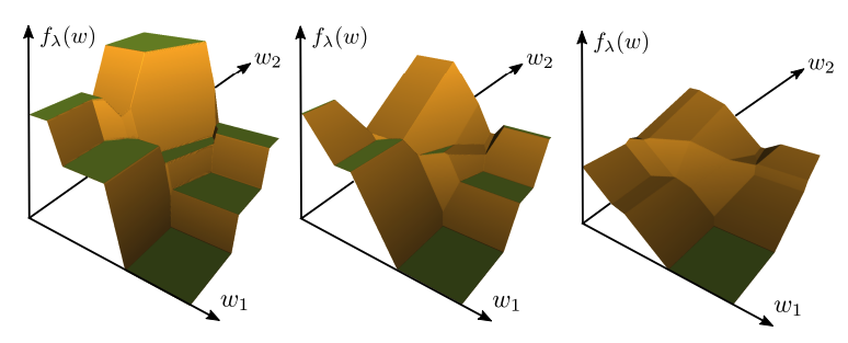
All of these intuitions are, of course, made rigourous and proved in the paper. Crucially, they generalize to high-dimensional \(w\), though that's harder to visualize. We can still do so for 2-dimensional \(w\), an example of which is pictured below. Moving from left right, we see how increasing \(\lambda\) causes \(f_\lambda\) to be less faithful to the piecewise constant \(f\), but provides a reasonable gradient on a larger set.
The authors present proof-of-concept experimental results, where they successfully train the proposed architecture on several synthetic tasks of realistic size. All of the tasks take images as raw input, extract suitable features, then use a blackbox solver to compute the optimal solution to an underlying combinatorial optimization problem.
As a baseline, the authors compare against a ResNet18 architecture, trained to directly predict the optimal solution to the optimization. The comparison is meant to illustrate the benefit of imposing inductive bias by directly modeling the optimization component. A vanilla architecture could conceivably learn representations that successfully produce the optimal solution \(-\) however, given the complex combinatorial structure we don't expect that they will in practice, and indeed they don't.
The first experimental task relates to the shortest-path problem we used as a running example earlier. As depicted below, the input \(x\) is a screenshot of a Warcraft 2 terrain map, where we wish to find the shortest path from the top-left to the bottom-right corner.
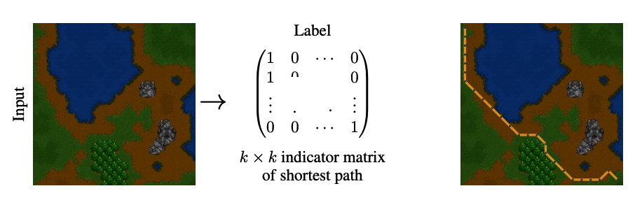
The maps have an underlying grid of dimension \(k \times k\), where each vertex corresponds to a terrain tile with (unknown to the network) cost. The architecture first uses convolutional and pooling layers to output a \(k \times k\) grid of predicted vertex costs, then computes the shortest path using Dijkstra's algorithm with the predicted costs. The loss is the Hamming distance of the proposed path from the true shortest path, calculated using the true grid costs.
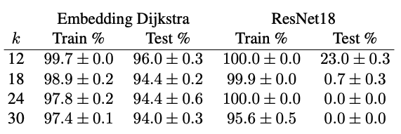
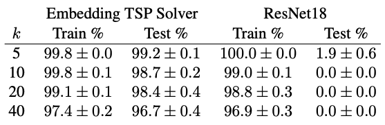
The results, given in the table below, show that the trained architecture achieves high accuracy on both the training and test sets. On the other hand, while the ResNet18 is able to memorize the training examples, it and utterly fails to generalize (as expected).
The second task is a bit more interesting, in that it also allows the authors to test whether the pre-solver architecture extracts useful representations. Here, the input \(x\) consists of \(k\) randomly selected country flags. The goal is to produce a travelling salesman tour through the capitals of the corresponding countries, minimizing total travel distance:
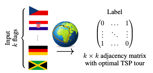
The architecture first uses convolutional layers to produce \(k\) three-dimensional vectors, which are then projected on to the unit sphere in \(\mathbb{R}^3\) that represents the globe. The pairwise distances on the manifold are passed to a TSP solver that produces a tour, and loss once again minimizes Hamming distance from the optimal tour using the true capital locations. The accuracy results are very similar to before:
More interestingly, we can visualize where the network thinks the world capitals are located by looking at the learned representations:

Keep in mind that the only information that the network saw was pictures of the countries flags' and the order that they would be visited under the optimal tour. Just from this it was able to place their capitals on a map (up to a rotation).
In my opinion, these proof-of-concept results show great promise. They tackle problems of realistic size, illustrate the end benefits of a hybrid optimization architecture, and are just plain cool. It would of course be very interesting to see the method applied to a real application like routing or object detection. I would also be remiss if I didn't mention that the authors have published easy-to-use PyTorch code exists for the project and experiments.
With that, I hope you found this work as exciting as I did and see you around!
[1] Vlastelica, Marin, Anselm Paulus, Vít Musil, Georg Martius, and Michal Rolínek. "Differentiation of blackbox combinatorial solvers." arXiv preprint arXiv:1912.02175 (2019).
[2] Boeing, Geoff. "What's New with OSMnx, Part 1." Online, 2020. Accessed Dec. 3, 2021. https://geoffboeing.com/2020/06/whats-new-with-osmnx/.
[3] Elmachtoub, Adam N., and Paul Grigas. "Smart “predict, then optimize”." Management Science (2021). Preprint.
[4] Williams, H. Paul. Model building in mathematical programming. John Wiley & Sons, 2013. Chapters 7-10.