GANs for Sequence Modeling

09 Dec 2021 | nlp rl gans Roger Jin

Today we’ll be trying to demystify the SeqGAN paper. We’ll go over

• Why we might want to use GANs for sequence modeling,
• Why we can’t apply GANs to sequence modeling directly,
• And how we can reformulate sequence modeling with reinforcement learning to get past this barrier.

Reviewing RNNs

Let’s remind ourselves of how language modeling is typically done these days. We have some prefix of words $w_1,\ldots,w_{n}$ and we want to generate $w_{n+1}$, so in particular we want to learn the conditional distribution

\[\begin{equation} P\left(w_{n+1} | w_1, \ldots, w_{n}\right)\\ \end{equation}\]

for every $w_{n+1}$ in our vocabulary $V$. If we know this conditional distribution, one reasonable $w_{n+1}$ to choose might be

\[\begin{equation} \underset{w_{n+1} \in V}{\arg \max}\hspace{0.1cm} P\left(w_{n+1} | w_1, \ldots, w_{n}\right). \end{equation}\]

In practice, we approximate this conditional distribution for every word $w_{n+1}$ and for every prefix $w_1,\ldots,w_{n}$ by a language model (LM), which consumes the prefix words $w_1, \ldots, w_{n-1}$ and passes them to an encoder to generate a hidden state $h_{n-1}$, a vector representation of the prefix. RNN language models will consume the prefix words one at a time, while transformer language models will consume them all at once. The language model then passes $h_{n-1}$ along with $w_n$ through a decoder to generate a vector of scores (logits) $s_1, \ldots, s_{| V |}$, one for each word in the vocabulary $V$. These scores can then be passed through a $\operatorname{softmax}$ to get squashed into probabilities to arrive at a predicted conditional distribution \(\begin{equation} \hat P\left(w_{n+1} | w_1, \ldots, w_{n}\right). \end{equation}\)

During training, $w_1,\ldots,w_n, w_{n+1}$ are consecutive words from our dataset and we penalize the model by the negative log likelihood loss

\[\begin{equation} L(w_1, \ldots, w_n, w_{n+1}) = -\log \hat P\left( w_{n+1} | w_1, \ldots, w_n \right). \end{equation}\]

Now suppose we have a trained LM and we want to generate text from it (we call this inference). We can do this by generating one word at a time and appending to a prefix which we condition on to get the next word, feeding outputed words back into our LM autoregressively to get new next words. To keep things simple, suppose we use a greedy decoding - that is, at each step, we take $\arg \max$ over the output probability distribution (or equivalently output logits) to choose the next word. We then have the relation

\[\begin{equation} w_{n+1} = \arg \max \operatorname{LM}(h_{n-1}, w_n), \end{equation}\]

recalling that $h_{n-1}$ is a hidden state representing the prefix $w_1, \ldots, w_{n-1}$.

Thus, during training, the input prefixes come from the data, while during inference, they come from the outputs of the model.

Problems

RNNs are unreasonably effective. At the very least, they might be better at blog writing than this poor author. However, they are not devoid of weaknesses.

Problem: Exposure bias

Recall that we have a distribution shift between training and inference - during training, inputs come from the data, while during inference, inputs come from the outputs of the model. We call this problem exposure bias - the model is never exposed to its own output during training, and so during inference with every successive word we add to the prefix from the model output, the generated text distribution drifts further from the data text distribution.

Of course, one solution is to expose the model to its own input during training (this is known as scheduled sampling). However, briefly, the problem with this approach is that the label for an input still comes from the data, so if the model generates “I like eating chicken,” the next word the model generates might be “nuggets,” which is perfectly reasonable. However, the excerpt from the text may have in fact been “I like eating elderberry jam”, in which case “nuggets” is a ridiculous answer to the data prefix “I like eating elderberry”. We’ll come back to the exposure bias problem shortly.

Problem: Penalizing full generations

In traditional LM training, the penalties are assigned word by word - given a prefix from the data, maximize the predicted likelihood of the next word from the data. However, this chained generation strategy does not assign any penalty holistically to the entire generation. And in fact for greedily decoded generations, backpropagating a holistic penalty is futile.

Recall that in greedy decoding, we generate a piece of text word by word in sequence and pick the next word by taking an $\arg \max$ over the $| V |$ logits in the output layer of our LM, where $\arg \max (\mathbf x)$ gives us the index of $\mathbf x$ of greatest value. Taking zero-indexing to be the convention, $\arg \max([7, 10]) = 1$. The below figure shows a plot of $z = \arg \max(x, y)$. Try hovering your cursor over the figure. Do you notice any problems this might cause for gradient updates?

The problem is that $\arg \max$ is locally constant! That is, its gradient is 0 almost everywhere. And so with traditional LMs under greedy decoding, penalties assigned to entire generations lead nowhere (was tempted to write “nowhere almost everywhere” but held my tongue).

Wait but why didn’t we have this problem of differentiating through an $\arg \max$ with traditional LMs? Since during training our prefixes come from the data (and not autoregressively from the $\arg \max$ of the output logits), there’s never a need to take a derivative of an $\arg \max$.

GANs to the rescue?

With some wishful thinking, we might think about trying to deal with the exposure bias problem with Generative Adversarial Networks (GANs). After all, GANs are designed to learn the distribution of the data and sample from it. So suppose that we have a text generator (aka a language model) $\operatorname{LM}$ and a text discriminator $D$ that attempts to assigns a score to a text input proportional to the likelihood the text input comes from the real world. The discriminator tries to maximize the realness scores it assigns to real text examples and minimize the realness scores it assigns to generated text examples, while the generator tries to minimize the realness scores the discriminator assigns to generated text examples. And so we can naturally define the following loss for an LM generation $w_1,\ldots,w_n$

\[\begin{equation} L(w_1,\ldots, w_n) = -\log\left(1 - D(w_1,\ldots,w_n)\right) \end{equation}\]

We quickly realize we have a problem - the discriminator loss is on full generations from $G$, and as we already know, that leads to problems under greedy decoding. In fact, even if we could pass nonzero gradients back through our generations, our setup still wouldn’t work.

That’s because language generation is inherently different from image generation. If we’re doing image generation and the gradient of our discriminator loss says pixel $(43, 172)$ should get its red value bumped up from its present value of $32.7$, then $32.7 + \varepsilon$ lands us at another shade of red. In contrast, if we’re doing language generation and the gradient of our discriminator loss is giving us a perturbation on the 7th word (say it’s penguin), then penguin + 0.001 doesn’t give us another word.

Are we doomed?

Reinforcement learning to the rescue

If we broaden our view a little bit, we might remember that there’s a whole field of machine learning devoted to sequential decision making - turn left, go straight, stop at the light. Knight e4, opponent takes, take back with the bishop. How do the reinforcement learning guys sleep at night with all of those $\arg \max$’s in their code?

In short, the answer is that we’re allowed to use $\arg \max$’s if we do some random sampling for the steps that come after the $\arg \max$.

Justification for this comes from the policy gradient theorem, which says that for a stochastic policy $\pi_\theta$ (parameterized by $\theta$), under certain regularity conditions,

\[\nabla_\theta \mathbb E_{\tau \sim \pi_\theta} \left[ R(\tau) \right] = \mathbb E_{\tau \sim \pi_\theta} \left[ \sum_{t=0}^T \nabla_\theta \log \pi_\theta (a_t | s_t) R(\tau) \right].\]

Why might this be useful? Our objective in RL is to maximize expected reward. Ideally, we would like to do this by gradient ascent, but \(\nabla_\theta \mathbb E_{\tau \sim \pi_\theta} \left[ R(\tau) \right]\) is a bit of a mysterious object to compute directly (gradient of an expectation w.r.t. the parameters of the underlying distribution?). Luckily for us, if we’re allowed to swap derivatives and integrals (this is where the regularity conditions come in), then we can write the gradient of an expectation as the expectation of a gradient. The gradient in the R.H.S., \(\nabla_\theta \log \pi_\theta\) is a straightforward computation. And via the law of large numbers, we can estimate the expectation in the R.H.S. by simulating a bunch of episodes $\tau \sim \pi_\theta$, computing gradients, and then taking their mean. This sort of simulation is known in fancier terms as Monte Carlo search.

Note that in particular, $R(\tau)$ is the reward for a full episode(!).

Reframing language modeling as RL

We’re ready to apply the trade secrets we pillaged from the RL people. There’s a very natural reformulation language modeling as a reinforcement learning problem. Again we generate word by word in order. States are prefixes, actions are next words, episodes are full generations, and the reward for a full generation is how well we fool the discriminator. The following figure from the SeqGAN Paper illustrates how all the moving pieces we discussed come together in training.

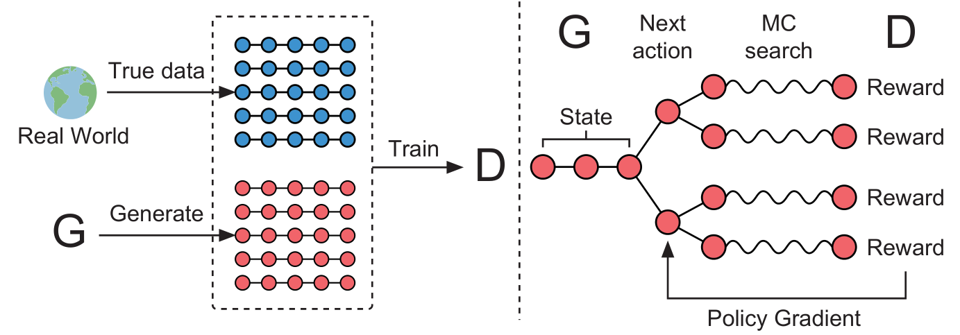
The generator (an RNN language model) samples full generations which are fed into a discriminator, which produces rewards representing how real the generations look. Each gradient is computed as a linear combination of of log-policy gradients, with coefficients given by the rewards.

So how exactly did we get around the need to differentiate through an $\arg \max$? In short, instead of decoding greedily, we decoded by random sampling.

Wait but isn’t taking the derivative of a sampling operation even more mysterious? The answer is that we don’t have to do this, because we no longer pass gradients from discriminator to generator. Note that even though we have a reward function, in generator training we’re not taking its derivative. The reward is simply an observation we make from our environment - from the generator’s perspective, it’s not part of our model. The trick is for each generation (episode), we pretend that we chose all of the next words (actions) correctly, compute gradients based on these guessed labels, and then weight those gradients based on the reward the generation (episode) produces.

And that’s pretty much it. Those are the basic ideas from the SeqGAN Paper.

New Problems

Since we’re using GANs, we inherit all the problems that come with GAN training - instability, mode collapse, vanishing gradients, and so forth. And since we’re using RL, we also inherit all the problems that come with RL - credit assignment, reward sparsity, high compute cost, and so forth. These problems are compounded by the fact that the action space is enormous - equal to the size of the vocabulary, for state of the art English LMs this is on the order of $50,000$. It is difficult to even imagine other RL problems with such a large action space. In comparison, the board size in Go is $19 \cdot 19 = 361$ possible points on which to lay a stone.

Why might this be useful?

Sure the exposure bias problem is aesthetically unpleasing, but incredibly powerful language models have been built training on next-word prediction alone. So then why would anyone ever go through the trouble of training an RL agent for language modeling? Again the answer lies in the ability to penalize a full generation. Suppose that we have a model that can give a text input a score proportional to how funny it is. If we want to tune our language model to be funnier, backpropagating through an $\arg \max$ isn’t an option, but treating funniness score as a reward function and sampling a bunch of generations to apply the Policy Gradient Theorem is.