Over-squashing in Graph Neural Networks

09 Dec 2021 | graph neural networks over-squashing over-smoothing Balla, Julia

Graph Neural Networks (GNNs) have achieved great success in modelling complex relational systems. They have been applied to graph-like data in a wide range of domains from molecular structures to social networks.

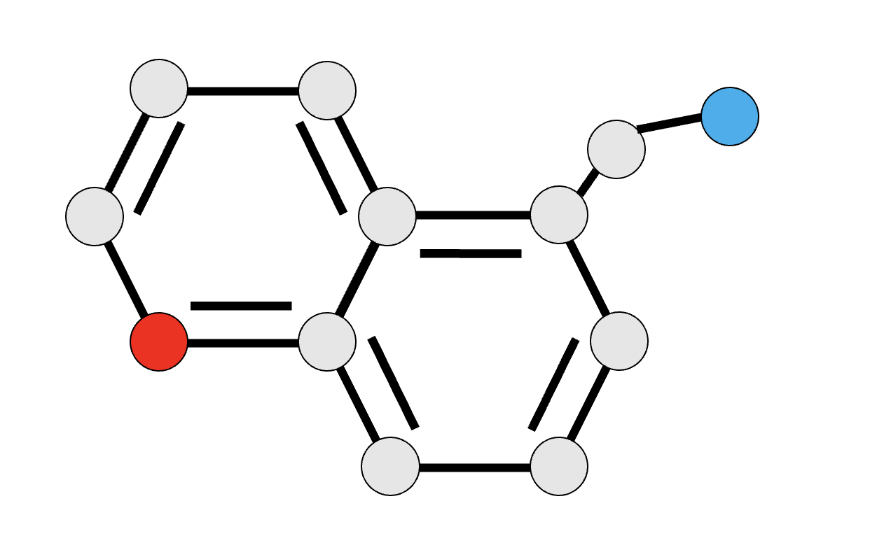
However, GNNs often struggle with efficiently propagating information over long distances on graphs. They have empirically been shown to exhibit a significant drop in performance beyond just 3-4 layers. This is a significant issue as there are many real-world graph learning tasks that depend on long-range signals. For instance, the prediction of a molecule’s properties may require compiling information from atoms on opposite ends [1].

The recent paper “On the Bottleneck of Graph Neural Networks and its Practical Implications” by Uri Alon and Eran Yahav identifies a new explanation for the inefficient flow of information between distant nodes, called over-squashing [2]. This blog post will discuss the phenomenon of over-squashing as defined in the paper, its relation to other measures of information loss in GNNs, and some proposed solutions.

1. What is over-squashing?
2. Over-squashing in practice
   • A synthetic experiment
   • Existing models
3. Over-squashing vs. over-smoothing
4. How can we squash the problem?
5. Conclusion
6. References

What is over-squashing?

Most GNNs rely on the message-passing framework [1], in which node representations are generated by aggregating information from neighboring nodes at each layer. This framework works especially well for short-range tasks where the desired output at a given node depends mostly on nodes that are a few hops away. The farthest distance that information needs to travel is referred to as the problem radius. The number of layers in a GNN must thus be greater than or equal to the problem radius for a given task.

In long-range tasks with a large problem radius, information must be propagated over many layers. At each step, the node representations are aggregated with others before being passed along to the next node. Since the size of the node feature vectors doesn’t change, they quickly run out of representational capacity to preserve all of the previously combined information. Over-squashing occurs when an exponentially-growing amount of information is squashed into a fixed-size vector.

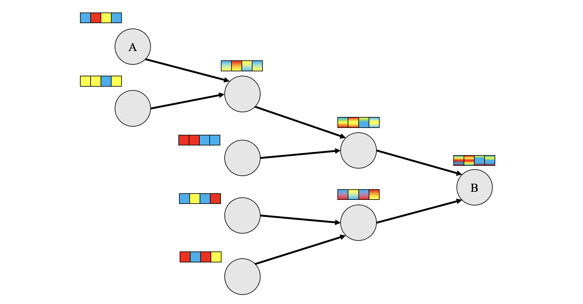
For example, in the diagram below, information from node A and other nodes along the propagation path must be squashed into a fixed-size vector before reaching node B. This type of graph structure gives rise to an information bottleneck at B.

We’ve seen the intuition behind over-squashing, but how prominent is the issue in practice?

Over-squashing in practice

The paper first studies over-squashing through a controlled experiment on a synethetic graph task, before working with existing datasets and GNN models.

A synthetic benchmark

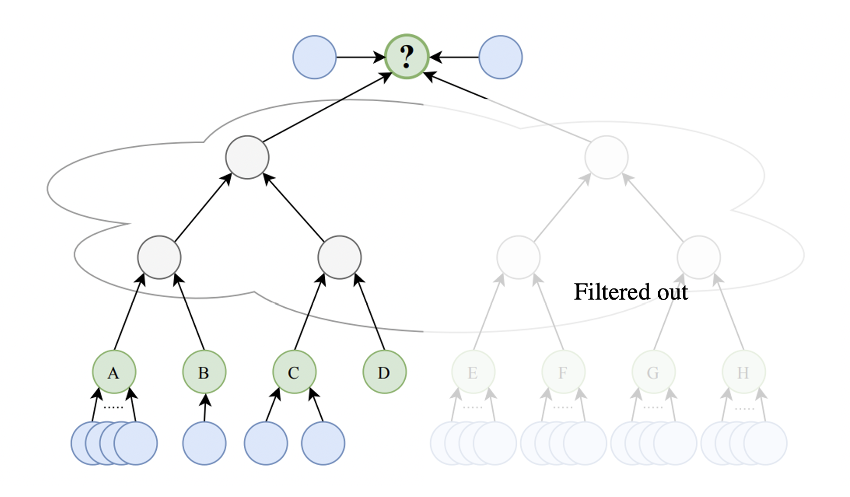
To compare the effects of over-squashing in several GNN variants, the authors contrived a graph learning task called the NeighborsMatch problem. The NeighborsMatch graph consists of two main types of nodes: green and blue. Green nodes have alphabetical labels and a varying number of blue neighbors. There is also one green target node. The objective is to predict the label of the green node which has the same number of blue neighbors as the target.

The experiments were run using a special instance of the NeighborsMatch problem known as Tree-NeighborsMatch.

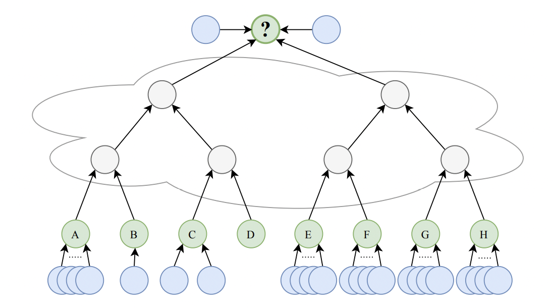
Consider the above example from the paper. The green nodes are labeled A-H, and the target node is labeled ‘?’. The grey nodes in the middle are arranged in the form of a binary tree of depth $ d=3 $. In this example, the correct prediction is ‘C’ because node C has the same number of blue neighbors as ‘?’.

To solve Tree-NeighborsMatch, information must be propagated from all of the green leaves to the target root. This means that the problem radius $ r $ is exactly equal to $ d $. We can therefore regulate the intensity of over-squashing by changing the depth of the tree.

Using this task for the experiments, the paper analyzes the effects of increasing the problem radius on the training accuracy as opposed to test, thus measuring the ability of the GNN to fit the input data. The GNN variants studied are:

• Gated Graph Sequence Neural Networks (GGNN) [3]
• Graph Attention Networks (GAT) [4]
• Graph Isomorphism Networks (GIN) [5]
• Graph Convolutional Networks (GCN) [6]

As shown in the plot below, the impact of over-squashing depends on the architecture of the GNN.

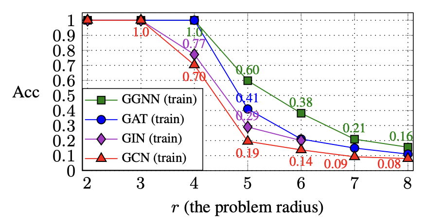
The key difference lies in the way each GNN aggregates the representations of neighboring nodes. For instance, GCNs and GINs squash all of the information being propagated from the leaves into a single vector before combining it with a target node’s representation. These architectures were only able to achieve 100% train accuracy up to a problem radius of 3.

On the other hand, architectures like GAT use attention-based weighting of the incoming messages. This means that at each node in the binary tree, it can filter out the information incoming from the branch that contains irrelevant information.

The amount of information that needs to squashed is halved in this case, so we see better results with respect to GCN and GIN at a radius $ r $ that is larger by 1.

The authors also hypothesize that GGNNs perform very well because the Gated Recurrent Units (GRUs) perform a similar filtering to GAT using element-wise attention [7]. By using a more effective filtering sheme, GGNNs achieve greater training accuracy than the other architectures.

Existing models

Over-squashing was present in the Tree-NeighborsMath problem by design. How prominent is the issue for real-world GNN models? To measure the phenomenon, Alon and Yahav used the technique of modifying the last layer in several existing models to instead be a fully-adjacent layer (FA), where each node is connected to every other node.

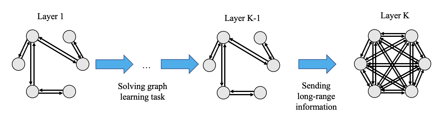
If there are $ K $ layers, only the first $ K-1 $ would be aware of the graph’s topology. This means that the first $ K-1 $ layers would no longer have to optimize for preserving long-range information, as this information would instead be passed along during the FA layer. The last layer would allow every node to directly communicate with one another and reduce the effect of the information bottleneck.

Note that the FA layer is not a proposed solution for the issue. It is rather an intentionally simple fix that acts as an indicator for the presence of over-squashing. The hypothesis is that if the FA layer modification leads to an improvement in the error rate, then this is evidence of over-squashing in the original model.

The augmentation of the last layer was indeed shown to cause a significant decrease in the error rate (42% on average) across six GNN variants. The paper concludes that since even a simple solution like the FA layer led to an improvement in extensively tuned models, over-squashing is very prevalent.

But what if over-squashing is only part of the problem? Could there be other explanations for the performance increase resulting from the FA layer? While the experiments with changing GNN parameters ruled out hyperparameter tuning as the culprit, a remaining candidate is the phenomenon of over-smoothing [8] in GNNs.

Over-squashing vs. over-smoothing

Over-smoothing is the related problem in which interacting nodes converge to indistinguishable representations as the number of GNN layers increases. This is a result of information between two nodes being combined and passed along back and forth over many iterations. An example is demonstrated below, where the mixing of colors represents the smoothing of node representations.

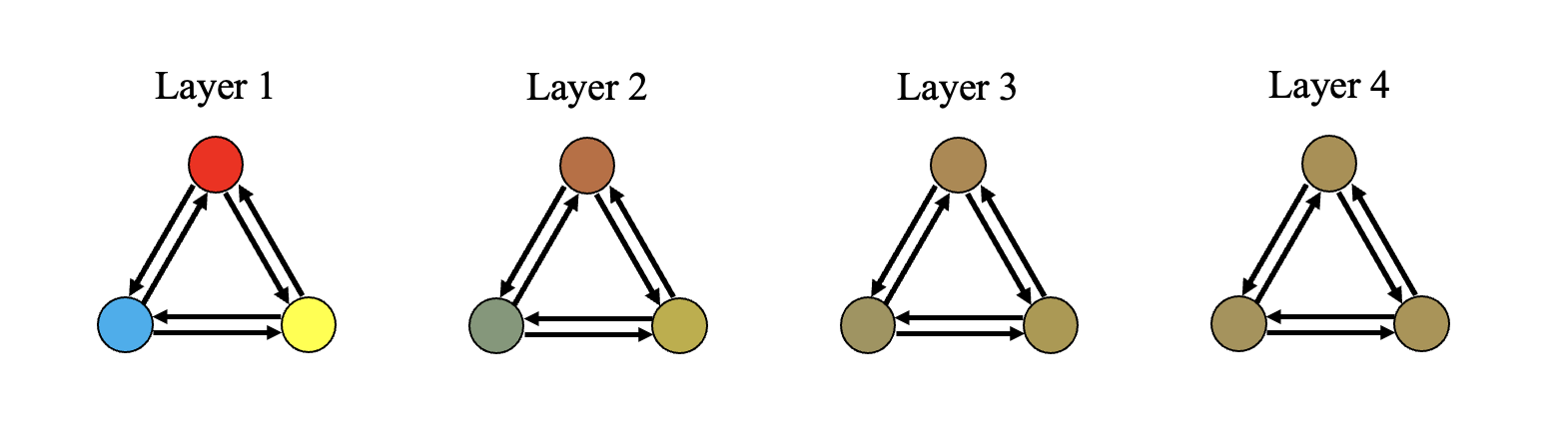
Over-smoothing intuitively seems very similar to over-squashing, and it is in fact the long-standing explanation for the poor performance of GNNs as the number of layers increases. However, the two phenomena are distinct. Over-smoothing occurs when the number of layers is much greater than the problem radius no matter how small the latter is. In the above example, the problem radius is 1 since the graph is fully connected, and the node representations already become difficult to distinguish by layer 3. However, information is not being condensed over long distances, so there is no over-squashing.

Over-squashing occurs when the problem radius is large and the number of layers is also at least as large (we may disregard the trivial case in which there aren’t enough layers for the GNN to solve the desired task). For instance, in the Tree-NeighborsMatch task with the number of layers matching the depth of the tree, the amount of information flowing into each parent node is double that of its child nodes. This is a case where there is over-squashing but no over-smoothing since the subtrees don’t interact and there aren’t enough layers to have two nodes converge to the same vector representation.

We may observe both phenomena when the problem radius is large and when the number of GNN layers is even larger. In this case, there seems to be no straightforward way to determine where most of the information loss would be coming from.

Going back to paper’s empirical results, it is then possible that over-smoothing was also present in models for the non-synthetic data to some extent. The chosen models all required a large number of layers when tuned to the given data, indicating that the problem radii were also large. By the above definitions, this does imply that over-squashing was likely the biggest issue. However, we do not know how the number of layers compare to the problem radius, so the effects of over-smoothing are unclear.

This raises the question of how to measure over-squashing and over-smoothing separately to better describe the information loss in GNNs: a promising direction of future research.

How can we squash the problem?

The following solutions are commonly used for improving the performance of GNNs on long-range tasks.

1. “Virtual” edges that connect distant nodes [1]. Adding these edges would allow information to flow directly between two nodes which were not previously connected, thus reducing the amount of information that must be squashed before reaching the target. Gilmer et al. tested this augmentation on GGNNs and found that there was a slight improvement in performance.

2. Master node [1]. A master node is connected to all other nodes by special edges and has its own representation vector for other nodes to send and obtain information. This effectively reduces the problem radius to 2, which diminishes the effect of over-squashing. This solution resulted in an even smaller error in GGNNs than adding virtual edges.

3. Skip connections [9]. Skip connections in GNNs “skip” some of the neighboring nodes when aggregating local information. Therefore, less information is being squashed at the aggregation steps. Skip connections have been shown to produce desirable results in GNNs.

All of the above solutions were developed without the explicit identification of the problem of over-squashing. This likely means that studying over-squashing more rigorously could lead to even better solutions and GNN methods.

A recent paper has been one of the first to do so through the lens of differential geometry [10]. Their findings led to a new graph-rewiring technique for mitigating over-squashing. For a high level overview, see the corresponding blog post referenced below [11].

Conclusion

Overcoming the problem of over-squashing is essential for improving GNN performance on tasks that require learning long-range signals. Some GNN variants suffer from over-squashing more than others depending on their information aggregation schemes. While there are a few simple GNN modifications that offer a partial solution to the problem, there is still much room for further improvements.

References

[1] J. Gilmer et al., Neural message passing for quantum chemistry. (2017) ICML.
[2] U. Alon and E. Yahav, On the bottleneck of graph neural networks and its practical implications. (2021) ICLR.
[3] Y. Li et al., Gated graph sequence neural networks. (2016) ICLR.
[4] P. Velickovic et al., Graph attention networks. (2018) ICLR.
[5] K. Xu et al., How powerful are graph neural networks? (2019) ICLR.
[6] T. Kipf and M. Welling, Semi-supervised classification with graph convolutional networks. (2017) ICLR.
[7] O. Levy et al., Long short-term memory as a dynamically computed element-wise weighted sum. (2018) ACL Volume 2: Short Papers, pages 732–739.
[8] Z. Wu et al., A comprehensive survey on graph neural networks. (2020) IEEE Transactions on Neural Networks and Learning Systems.
[9] K. Xu et al., Representation Learning on Graphs with Jumping Knowledge Networks. (2018) ICML.
[10] J. Topping, F. Di Giovanni et al., Understanding over-squashing and bottlenecks on graphs via curvature. (2021) arXiv:2111.14522
[11] M. Bronstein, Over-squashing, Bottlenecks, and Graph Ricci curvature. (2021) Blog post in Towards Data Science.