Transformer-powered Object Detection

Hello, world! DETR is a fascinating piece of work from Facebook AI. The authors develop a novel architecture that tackles the object detection problem using transformers. The focus of this post is the main idea of the paper. No results will be reported, as it will only hinder the readability. The full work (paper and code) is available here here.

Outline of this post:

1. Introduction
2. Matching and Training Loss
   • Matching Loss
   • Training Loss
   • Bounding Box Loss
   • Generalized IoU Loss
3. DETR Architecture
   • Object Queries
4. Conclusion

Introduction

The goal of object detectors is to generate a set of predictions for the bounding box and class of each object in the scene. Most modern object detectors perform this task indirectly. They make use of surrogate regression and classification tasks on a large set of proposals/anchors/window centers. Additionally, they requiring significant post-processing on their initial predictions in order to improve their quality (e.g., dropping duplicates and other heuristic methods).

This paper aims to simplify and streamline the object detection task by removing any hand-designed components, or prior knowledge about the task. This is achieved by using a set-based global loss that enforces unique predictions (via bipartite matching), and a transformer encoder-decoder network. The resulting model is able to perform parallel (non-autoregressive) prediction of the final set of detections (bounding boxes and class), using only common CNN and Transformer modules, readily available in most frameworks (note that the model also utilizes a pre-trained ResNet backbone, which is readily available in most frameworks as well).

Figure 1: This figure outlines the high level idea of the model architecture, and how the bipartite matching uniquely assigns predictions with ground truth boxes. Notice that the remaining predictions are assigned to the no object class. Duck image source.

Matching and Training Loss

The training task is split in to parts:

1. Matching the predictions to ground truth boxes.
2. Training based on the matching performed on the previous step.

Matching Loss

One of the major obstacles in training such a task is how to score predicted objects (position, size, class) with respect to the ground truth.

The model generates a fixed-size set of $N$ predictions, with a single pass through the transformer decoder. The number of predictions $N$ is significantly larger than the maximum number of objects possible in an image. In this work $N = 100$, and there’s no more than $63$ objects in a single image from COCO (on average there’s only 7).

The first step to solving this problem is through an optimal bipartite matching between predicted and ground truth objects. We are going to denote by $y$ the ground truth set of objects, and \(\hat{y} = \lbrace\hat{y}_i\rbrace_{i=1}^N\) the set of $N$ predictions. Under the assumption that $N$ is larger than the number of objects to be detected, we can consider that $y$ is also of size $N$, padded with \(\varnothing\) (no object) objects. Thus, the problem of finding a bipartite matching between the two sets boils down to finding the permutation $\sigma \in \mathcal{C}_N$ of $N$ elements that achieves the lowest cost:

where \(\mathcal{L}_{\text{match}}(y_i, \hat{y}_{\sigma(i)})\) is a pair-wise matching cost between ground truth $y_i$ and a prediction with index \(\sigma(i)\). The optimal assignment can be efficiently computed with the Hungarian algorithm. Code for this is readily available in python here.

The matching cost accounts for both the class and the similarity of the bounding boxes between prediction and ground truth. Each element $y_i$ can be seen as \(y_i=(c_i, b_i)\) where $c_i$ is the class label (note that it can be $\varnothing$) and $b_i \in [0, 1]^4$ is a normalized vector encoding the center of the bounding box, and its width and height. Further, for a prediction $\hat{y}_{\sigma(i)}$ we define probability of class $c_i$ as \(\hat{p}_{\sigma(i)}(c_i)\) and predicted bounding box as \(\hat{b}_i\). Following these notations, we can now define the matching cost as:

where \(\mathbf{1}_{\lbrace c_i\neq\varnothing\rbrace}\) is an indicator function that equals to $1$ when $c_i\neq\varnothing$ and $0$ otherwise. Also, \(\mathcal{L}_{box}\) is a loss functions that measures how similar two bounding boxes are (the more similar, the lower the loss). Notice how the matching loss is $0$ for all the $i$ s.t. $c_i=\varnothing$. That is because we care about assigning a non empty class and true bounding box only to a small subset of all our predictions. The rest predictions are automatically assigned to the no object class (but their is no bounding box assignment).

Training Loss

Having solved the matching problem, we should have an optimal assignment based on the matching loss. Thus, we can now define the Hungarian loss (this is the training loss) for all pairs matched. The Hungarian loss is very similar to how most object detectors define their loss, i.e., a linear combination of a negative log-likelihood loss for the class and a box loss (the same one used in the matching loss, which we will define later) for the bounding boxes:

where $\hat{\sigma}$ is the optimal matching from the previous step. There are several things we need to note here.

1. In practice we down-weight the log-probability term when $c_i=\varnothing$. This balances the effect of training between positive and negative proposals (on average there’s only 7 objects in each image, but we generate 100 proposals).
2. In the training loss we drop the indicator function in front of the classification term (while we need it there for the optimal matching task). This is because now we actually want to teach the model to only assign a positive class to ‘real’ objects, and negative (no object, $\varnothing$) to everything else.
3. Note how for the proposals that are matched to $\varnothing$ there is no gradient pushed back for the bounding box prediction task. That’s because we only care that the model marks them as no object, but we don’t really care where it places them.
4. Note how in the training loss we use negative log-likelihood for the classification loss, however, we just used the negative probability for the matching loss previously. The reason we want to do that for the matching loss is because log-likelihood can take very large values compared to $\mathcal{L}_{box}$. Thus, using the probability as is leads to better assignments (especially in the early iterations where the classification loss can be very large), and better empirical performances.

Bounding Box Loss

Finally, we will discuss the bounding box loss, \(\mathcal{L}_{\text{box}}(b_i, \hat{b}_{\hat{\sigma}(i)})\). Since we are directly predicting the bounding boxes, without making use of any anchors/initial guesses, the implementation is simplified, however, relative scaling becomes an issue. Specifically for $\mathcal{l}_1$ loss, bigger bounding boxes will have different scale than smaller ones, even if the relative error is similar. To offset this shortcoming, the authors use a linear combination of the \(\mathcal{l}_1\) and the Generalized IoU loss \(\mathcal{L}_{\text{iou}}(\cdot, \cdot)\):

Note that the above loss is normalized by the number of objects inside the batch.

Generalized IoU Loss

At this point it would be good to give a brief explanation on the Generalized IoU, or GIoU. GIoU is an extension of the standard IoU that takes care of the cases where the two bounding box are disjoint. When the bounding boxes are disjoint, the standard IoU is $0$, thus, it doesn’t provide any gradient to improve the predictions, so learning/convergence is slower as we have to rely only on the $\mathcal{l}_1$ loss. GIoU on the other hand extends IoU by taking into account the difference between the area of the convex hull of the two sets, and the area of the union. In strict mathematical notation, for two sets $A$ and $B$, this can be written as:

where $C$ is the smallest convex hull of $A$ and $B$.

Figure 2: GIoU vs IoU demonstration. Notice how, IoU is $0$ when the two boxes don’t overlap, giving no gradient to train on. Also, note how even when they overlap there is still some difference between IoU and GIoU. Only when there is complete overlap ($A \subset B$ or $B \subset A$) the two metrics are matching (because $C=A\cup B$).

Thus, we define:

One could also try other IoU inspired metrics such as the Complete IoU, or the Distance IoU. For more information look here.

DETR Architecture

The proposed architecture is quite simple. It consists of a pre-trained CNN backbone (e.g., ResNet) to extract meaningful features, an encoder-decoder transformer, an FFN for the classification task, and an FFN for the bounding box task. Fig. 3 demonstrates at a high level how the model operates.

Figure 3: Schematic representation of how the DETR architecture works.

The listing below demonstrates the simplicity of this architecture as we can define the model in less than 40 lines of python code.

import torch
from torch import nn
from torchvision.models import resnet50

class DETR(nn.Module):

    def __init__(self, num_classes, hidden_dim, nheads,
        num_encoder_layers, num_decoder_layers):
        super().__init__()
        # We take only convolutional layers from ResNet-50 model
        self.backbone = nn.Sequential(*list(resnet50(pretrained=True).children())[:-2])
        self.conv = nn.Conv2d(2048, hidden_dim, 1)
        self.transformer = nn.Transformer(hidden_dim, nheads,
        num_encoder_layers, num_decoder_layers)
        self.linear_class = nn.Linear(hidden_dim, num_classes + 1)
        self.linear_bbox = nn.Linear(hidden_dim, 4)
        self.query_pos = nn.Parameter(torch.rand(100, hidden_dim))
        self.row_embed = nn.Parameter(torch.rand(50, hidden_dim // 2))
        self.col_embed = nn.Parameter(torch.rand(50, hidden_dim // 2))

    def forward(self, inputs):
        x = self.backbone(inputs)
        h = self.conv(x)
        H, W = h.shape[-2:]
        pos = torch.cat([
            self.col_embed[:W].unsqueeze(0).repeat(H, 1, 1),
            self.row_embed[:H].unsqueeze(1).repeat(1, W, 1),
        ], dim=-1).flatten(0, 1).unsqueeze(1)
        h = self.transformer(pos + h.flatten(2).permute(2, 0, 1),
                             self.query_pos.unsqueeze(1))
        return self.linear_class(h), self.linear_bbox(h).sigmoid()

detr = DETR(num_classes=91, hidden_dim=256, nheads=8, num_encoder_layers=6, num_decoder_layers=6)
detr.eval()
inputs = torch.randn(1, 3, 800, 1200)
logits, bboxes = detr(inputs)

Listing 1: Short python code that implements the DETR architecture. Source: the original paper.

In practice, the authors use a slightly more complex piece of code, and they also modify the vanilla pytorch transformer code. Some of the modifications are:

1. The backbone learning rate is 10 times smaller than transformer learning rate. This helps with stability, and with the fact that the backbone is already trained, so it is just fine tuning at this point.
2. The authors use a 3 layer MLP for the bounding box head, instead of single FFN.
3. Instead of using learned positional encoding for the transformer encoder, the authors opt for 2D sinusoidal encoding.
4. The positional encodings of the transformer encoder are added at each encoder layer, instead of just the first one.
5. The object queries (positional encodings of the transformer decoder) are also added at each decoder layer.
6. The authors introduce an auxiliary loss, which is basically the same Hungarian loss we talked about before, but applied to all the intermediate decoder layers. This essentially allows the model to train each decoder layer on the same object detection task, and the authors noticed that the accuracy increased as a functions of the layer depth (the last decoder layer has the best performance, and the first has the worst). Note that when using the auxiliary loss, all decoder layers use the same FFN modules, and they also share a layer-norm to normalize the inputs before the FFNs, after each decoder layer.

Object Queries

It’s time to turn our attention to the object queries. Simply put, object queries are nothing more than “learned positional encoding” that we use as input to the transformer decoder.

However, they play a very important role for the object detection task.

As it turns out, each object query “specializes” in identifying objects at specific parts of the input image, and/or specific object shapes (e.g., tall objects, or wide objects). An example of this can be seen in Fig. 4 below. That’s also the reason why the authors use 100 object queries even though on average there’s only 7 (for COCO), and at worst there’s 63 (again for COCO).
Potentially, this is one of the ways the model manages to solve the object detection task end-to-end, without any hand-designed priors, or heuristics (dropping near duplicates, using anchors, etc.).

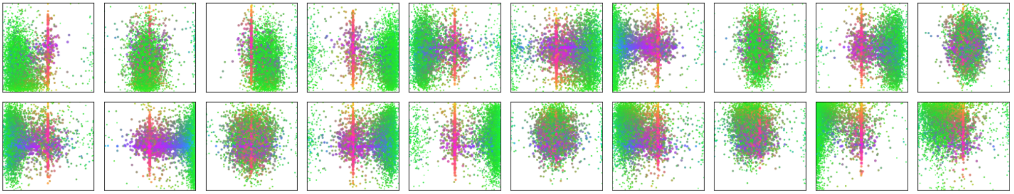Figure 4: Visualization of all box predictions on all images from COCO 2017 validation set for 20 out of total N = 100 prediction slots in DETR decoder. Each point represents the center coordinate of a predicted box (the coordinates are normalized by the image size, so everything lies on a 1x1 grid). Green points corresponds to small boxes, red to large horizontal boxes and blue to large vertical boxes. Source: the original paper.

Conclusion

The authors did a fantastic job with this paper. Their motivation to streamline the object detection task, by dropping all hand-designed heuristics, and prior knowledge, lead to a very interesting architecture, that can yield very strong results.

However, not everything is perfect with this architecture.
One of the issues with it is that it takes really long to train. Specifically, their best model took 500 epochs (where an epoch is a pass through all the training set once). This is because the attention maps start out uniform, and it takes really long until they become sparse and the transformer can actually learn where it needs to “look” at.
Another issue with DETR is that it performs poorly on smaller objects, even though it does very good on larger objects. This is because it uses a feature map extracted from ResNet that has much smaller resolution than that of the input image (width and height are reduced by a factor of 32).
A solution to these two problems is proposed in recent work that you can find here

There’s still plenty of material in the original paper that we didn’t cover, such as the model’s performance, extension of DETR for panoptic segmentation, etc. Thus, I would like to urge the readers to take some time to read the original paper.